
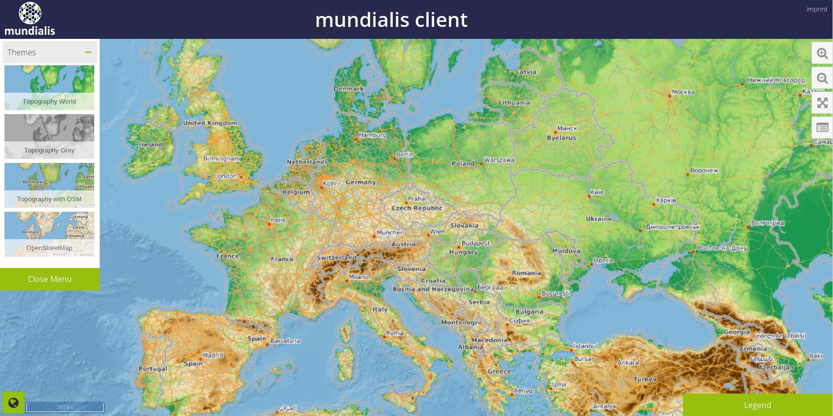
Imagine a new Web Map Service, that everybody can use in his desktop GIS or web application. It shows the topography of the earth in the background with an intuitive color range and useful information like cities, streets and country boundaries on top. It is fast and covers the whole world. In this post we explain how we made it for you. To see the result in action, just click the image below.
As we are very familiar and aware of the power of GeoServer, we decided to use it to publish our new services. As rendering of detailed and global data can become very time and performance consuming, we needed to speed up the serving of the imagery. Even powerful servers can’t cope with live rendering of massive datasets like OSM and high resolution DEMs in every possible resolution and extent while keeping the service fast and the user experience high. So we decided to use MapProxy to cache and speed up our new WMS. Each request to the service will either be served by the precalculated tile cache or, if the requested data is not available in the cache, calculated and afterwards stored in the cache. The combination of those two powerful Open-source software components enables you to create a nice looking and really fast WMS.
1. Topography Layer
The data
For our new layer we needed elevation data. We thought about the following options:
- ASTER 30m (570GB uncompressed, whole world)
- SRTM 30m (not available for whole world, should be ready in early 2016)
- SRTM 90m (size can be handled better, ~60GB for the whole world)
- SRTM 450m (~ 8GB, resolution fine when looking at the whole world, but not for large scales)
We already had ASTER GDEM data for Germany and a modified SRTM DEM 450m for the whole world, but we wanted to also use SRTM 90m data, because its file size and resolution is a reasonable compromise. The SRTM data by CIAT is supposed to be the best processed dataset available (SRTM v4.1 by CIAT, 14GB compressed, ~60GB decompressed) and consists of multiple GeoTIFF files. These files can be easily published in GeoServer with the help of the Image Mosaic extension. After publishing the data in GeoServer, we were able to have a first look at its quality, which was somewhat disappointing. The dataset has several unknown and big squares in the ocean with an equal height of 255m and the spatial extent in the northern and southern direction was too small to use it as a global dataset. So for now we use the modified SRTM DEM 450m with an ASTER-Overlay of Germany. We can add higher resolution data at anytime later from the ASTER dataset.
The style
The good thing about elevation data is that it usually tells the height in meters for each pixel. The property’s name for many raster datasets with only one band is called ‚GREY_INDEX‘ in GeoServer. This means, that we can use the same style for different elevation data. Our first step in creating a color-ramp was finding meaningful minimum and maximum values for the land topography. Mount Everest causes the highest elevation value with 8848m, the lowest value describes the surface of the Dead Sea which is -420m. As there are only few places in the world above 8000m, we decided to start to generalize above 6000m. This is where our colormap in the SLD ends (see below). It starts with a transparent value for 0m above sea level and below, because – depending on the dataset – these are the values for the surface of the sea, which we don’t want to display. But what happens to the places on land surface which are below 0? They will be transparent as well. So we put another layer behind our topography layer, containing polygons of land and color them like the value which is closest to 0m. So for now, we can’t distinguish in color between 0m and -420m above sea level. We may change this next time.
<ColorMapEntry color="#0f572e" quantity="-420" label="label" opacity="1"/><!-- darkest green-->
Between 0.1m and 6000m we build a colormap. As altitude rises, colors change from green, yellow, brown and dark grey to light grey:
<?xml version="1.0" encoding="ISO-8859-1"?>
<StyledLayerDescriptor version="1.0.0"
 xsi:schemaLocation="https://www.opengis.net/sld StyledLayerDescriptor.xsd"
 xmlns="https://www.opengis.net/sld"
 xmlns:ogc="https://www.opengis.net/ogc"
 xmlns:xlink="https://www.w3.org/1999/xlink"
 xmlns:xsi="https://www.w3.org/2001/XMLSchema-instance">
  <!-- a Named Layer is the basic building block of an SLD document -->
  <NamedLayer>
    <Name>default_raster</Name>
    <UserStyle>
    <!-- Styles can have names, titles and abstracts -->
      <Title>Default Raster</Title>
      <Abstract>A sample style that draws a raster, good for displaying imagery</Abstract>
      <!-- FeatureTypeStyles describe how to render different features -->
      <!-- A FeatureTypeStyle for rendering rasters -->
      <FeatureTypeStyle>
        <Rule>
          <Name>rule1</Name>
          <Title>Opaque Raster</Title>
          <Abstract>A raster with 100% opacity</Abstract>
          <!--<MinScaleDenominator>250000</MinScaleDenominator>-->
          <RasterSymbolizer>
              <Opacity>1</Opacity>
              <ColorMap type="ramp">
                  <ColorMapEntry color="#2166ac" quantity="0" label="label" opacity="0"/><!-- transparent-->
                  <ColorMapEntry color="#1a9850" quantity="0.1" label="label" opacity="1"/><!-- dark green-->
                  <ColorMapEntry color="#a6d96a" quantity="150" label="label" opacity="1"/><!-- light green-->

                  <ColorMapEntry color="#f6e8c3" quantity="500" label="label" opacity="1"/><!-- lightest brown-->
                  <ColorMapEntry color="#dfc27d" quantity="800" label="label" opacity="1"/><!-- light brown-->
                  <ColorMapEntry color="#bf812d" quantity="1500" label="label" opacity="1"/><!-- lighter dark brown-->

                  <ColorMapEntry color="#8c510a" quantity="2000" label="label" opacity="1"/><!-- dark brown-->
                  <ColorMapEntry color="#452805" quantity="3000" label="label" opacity="1"/><!-- darkest brown-->

                  <ColorMapEntry color="#878787" quantity="4001" label="label" opacity="1"/><!-- darkest gray-->
                  <ColorMapEntry color="#bababa" quantity="5001" label="label" opacity="1"/><!-- dark gray-->
                  <ColorMapEntry color="#e0e0e0" quantity="5501" label="label" opacity="1"/><!-- light gray-->
                  <ColorMapEntry color="#fafafa" quantity="6001" label="label" opacity="1"/><!-- lightest gray-->
              </ColorMap>
          </RasterSymbolizer>
        </Rule>
      </FeatureTypeStyle>
    </UserStyle>
  </NamedLayer>
</StyledLayerDescriptor>
The layer
As mentioned above, there is not just one topography layer. We use geoservers group layer to craft the topography layer out of different sources. These layers are:
- Bathymetry – Shows seafloor relief. Free data by Natural Earth Data. The style is shaded relief so it differs from the topography
- Land surface polygons colored in dark green – Fills gaps in topography for land below sea level
- SRTM 450m – Lowest resolution elevation layer with coverage for whole world
- ASTER 30m – High resolution elevation layer with small coverage
- (Possible: more layer with little coverage and high resolution)
- Bathymetry of great lakes by NGDC – Created own style (see below)
- Transparent Overlay – For large scales, individual pixels become visible at some point. To reduce this, we put a white transparent layer on top which covers the whole world. If the scale becomes larger, we reduce the transparency (or raise the opaqueness) of this layer a little bit. This is the most easiest way to create a fade-out effect
Lake Bathymetry colormap of style:
<ColorMap type="ramp">
        <ColorMapEntry color="#045a8d" quantity="-9999" label="label" opacity="0"/><!-- transparency because of ill data-->
        <ColorMapEntry color="#045a8d" quantity="-300" label="label" opacity="1"/><!-- dark blue-->
        <ColorMapEntry color="#2b8cbe" quantity="-200" label="label" opacity="1"/><!-- lighter dark blue-->
        <ColorMapEntry color="#74a9cf" quantity="-100" label="label" opacity="1"/><!-- darker light blue-->
        <ColorMapEntry color="#bdc9e1" quantity="-50" label="label" opacity="1"/><!-- light blue-->
        <ColorMapEntry color="#f1eef6" quantity="1" label="label" opacity="0"/><!-- near white blue - transparent because above lake surface-->
        <ColorMapEntry color="#000000" quantity="8000" label="label" opacity="0"/><!-- transparent-->
</ColorMap>
Now we’ve created a topography layer with land elevation, sea and lake bathymetry. For better performance we use MapProxy and configure caching for scales smaller than 1:215.000. We configure which zoom levels to cache by setting the corresponding resolutions in MapProxy’s configuration file. If a request does not hit a cached resolution, MapProxy will stretch or shrink the next best resolution to serve the desired request. For scales larger than 215.000, the pixels become more and more visible, as this is the limit of the datasets resolution. MapProxy will use the last available cached resolution and stretch the image for the ouput, as GeoServer cannot deliver better quality anymore at this point. We seed the whole configured cache once, so with each request only tiles from the cache are served to the user.
Excerpt of mapproxy.yaml with important code for topography layer:
layers:
  - name: TOPO-WMS
    title: Topographic WMS - by mundialis
    sources: [topo_world_cache]

caches:
  topo_world_cache:
    grids: [topo_grid]
    sources: [topo_world_wms]
    image:
      format: image/png
      mode: P
      transparent: false
      encoding_options:
        quantizer: fastoctree
      resampling_method: bicubic
    link_single_color_images: true

sources:
  topo_world_wms:
    type: wms
    req:
      url: https://localhost:8080/geoserver/osm/wms?
      layers: topography
    wms_opts:
      featureinfo: true
    coverage:
      bbox: [-180, -88, 180, 88]
      srs: 'EPSG:4326'
    supported_srs: ['EPSG:4326']
    supported_formats: ['image/png8']
    concurrent_requests: 4
    http:
      client_timeout: 600

grids:
  topo_grid:
    tile_size: [256, 256]
    srs: 'EPSG:900913'
    res: [156543.03390625, 78271.516953125, 39135.7584765625, 19567.87923828125, 18000, 4891.9698095703125, 2445.9849047851562, 1222.9924523925781, 611.4962261962891, 305.74811309814453, 264.58333360, 152.87405654907226, 132.29166680, 76.43702827453613]
Excerpt of seed.yaml for seeding the topography layer once:
seeds:
  topo_world:
    caches: [topo_world_cache]
    grids: [topo_grid]
    levels:
      from: 0
      to: 13
2. OSM Overlay
The new topography-layer is a background layer without any further information like names, streets or lakes. To add that information we create a new group layer in geoserver from the OSM data. We copy most things from the terrestris OpenStreetMap-WMS which already exists. We remove the land-usage polygons, so the new overlay will have transparent areas, where instead the topography layer will be visible. One problem appears: the part of lake Superiour which is in Canada is visible, but not the part in USA. Analyzing OSM data tells us, that the tags used in the OSM data of the polygons differs. The OSM-WMS solves this problem by adding a blue background. In our case the topography lays behind, so this would not be a solution. As only lake Superiour is divided in half, we set it invisible in the style. Except the waterareas-style, we use the styles from the original OSM-WMS and also its ordering. We also cache this layer via MapProxy, but with more resolutions configured to allow detailed views in lower scales without live rendering through GeoServer.
3. Putting it all together
Both group layers are cached seperately. This has some advantages:
- The topography background doesn’t need updates frequently. Heights in the world do not change every month. When we add a high resolution dataset, we can start the calculation of the cache manually
- OSM-Overlay needs to be updated frequently, as this changes and needs to be up-to-date
- For the raster-topo layer, large scale resolutions don’t need to be calculated, as pixels are visible sooner or later
- For the OSM-vector layer, large scale resolutions need to be calculated
- Last but not least, having those layers cached seperately allows one to use the Overlayer-layer together with other background services, or just the plain Topographic WMS
To finally put both layers together, no additional geoserver group layer is needed, but simply a new MapProxy configuration, which uses two sources for a new layer. So the final layer is a composition of two independent and seperately cached layers, which solves the problems with different update intervals while preserving the overall speed through efficient caching.
layers:
  - name: TOPO-OSM-WMS
    title: Topographic OSM WMS - by mundialis
    sources: [topo_world_cache, osm_world_overlay_cache]
4. Sources
- Modified SRTM 450m by viewfinderspanorama
- ASTER GDEM 30m by Nasa GDEM
- Natural Earth Data
- Great Lakes Bathymetry by NGDC
- OSM
5. Where to find it
A client containing the layers is available here:
maps.mundialis.de
The Capabilities of the Wep Map Services are available here:
https://ows.mundialis.de/services/service?SERVICE=WMS&REQUEST=GetCapabilities
- Plain topography: „TOPO-WMS“
- OSM-overlay: „OSM-Overlay-WMS“
- Hybrid: „TOPO-OSM-WMS“